Predict CO2 Emission using Simple Linear Regression

 

Predict CO2 Emission using Simple Linear Regression

Introduction:

    In this blog, we learn how to use scikit-learn to implement simple linear regression on fuel consumption and Carbon dioxide emission of cars data. Then use model to predict unknown value.

    This blog offers you a step-by-step instruction guide with source code, so you can build your model. It is not designed to be a deep dive into model design, statistical analysis, improvement, and validation. If you want to learn more, please check out my blog site: Techy Scientists.

It contains the following parts:

1. Setup your environment
2. Data Preparation
3. Exploratory data analysis
4. Simple Linear Regression Model
5. Model Evaluation

Setup your environment

   To run the program on your local computer, install the following required libraries, These libraries are 

1.   python 3.8.0
2.   numpy
3.   pandas
4.   matplotlib
5.   scikit-learn

Data Preparation

Understand the data

  We have downloaded a fuel consumption dataset, FuelConsumption.csv, which contains model-specific fuel consumption ratings and estimated carbon dioxide emissions for new light-duty vehicles for retail sale in Canada. You can find more information about the data, go to Fuel consumption ratings.

• MODELYEAR e.g. 2014
• MAKE e.g. Acura
• MODEL e.g. ILX
• VEHICLE CLASS e.g. SUV
• ENGINE SIZE e.g. 4.7
• CYLINDERS e.g. 6
• TRANSMISSION e.g. A6
• FUEL CONSUMPTION in CITY(L/100 km) e.g. 9.9
• FUEL CONSUMPTION in HWY (L/100 km) e.g. 8.9
• FUEL CONSUMPTION COMB (L/100 km) e.g. 9.2
• CO2 EMISSIONS (g/km) e.g. 182 --> low --> 0

Import the Packages

  Create a python file (for example model.py). After installed the required packages and import packages  in your python file.

import numpy as np
import pandas as pd
import matplotlib.pyplot as plt
%matplotlib inline

Read the Data

  Read the data using Pandas

df = pd.read_csv('FuelConsumptionCo2.csv')

Information of the Data

    Information about given data,

df.info()

RangeIndex: 1067 entries, 0 to 1066
Data columns (total 13 columns):
MODELYEAR                   1067 non-null int64
MAKE                        1067 non-null object
MODEL                       1067 non-null object
VEHICLECLASS                1067 non-null object
ENGINESIZE                  1067 non-null float64
CYLINDERS                   1067 non-null int64
TRANSMISSION                1067 non-null object
FUELTYPE                    1067 non-null object
FUELCONSUMPTION_CITY        1067 non-null float64
FUELCONSUMPTION_HWY         1067 non-null float64
FUELCONSUMPTION_COMB        1067 non-null float64
FUELCONSUMPTION_COMB_MPG    1067 non-null int64
CO2EMISSIONS                1067 non-null int64
dtypes: float64(4), int64(4), object(5)
memory usage: 108.5+ KB

Missing Values

    Find the missing values of given data,

missing_values = df.isnull().sum()
missing_values[0:13]

ENGINESIZE                  0
CYLINDERS                   0
FUELCONSUMPTION_CITY        0
FUELCONSUMPTION_HWY         0
FUELCONSUMPTION_COMB        0
FUELCONSUMPTION_COMB_MPG    0
CO2EMISSIONS                0
dtype: int64

Exploratory data analysis

    Lets start exploratory data analysis on our data. First plot each of these features vs the Emission, to see how linear is their relation.

ENGINESIZE vs CO2EMISSIONS

CYLINDERS vs CO2EMISSIONS

FUELCONSUMPTION_CITY vs CO2EMISSIONS

FUELCONSUMPTION_COMB vs CO2EMISSIONS

FUELCONSUMPTION_COMB_MPG vs CO2EMISSIONS

FUELCONSUMPTION_HWY vs CO2EMISSIONS

    We don't consider irrelevant data points in linear regression. (Eg: Fuel consumption_comp_mpg is non-linear). So we decided to remove Fuel consumption_comp_mpg feature.

df.drop('FUELCONSUMPTION_COMB_MPG', 
	axis=1, 
    	inplace=True)

Simple Linear Regression Model

    Linear Regression fits a linear model with coefficients 𝜃=(𝜃1,...,𝜃𝑛)θ=(θ1,...,θn) to minimize the residual sum of squares between the independent x in the dataset, and the dependent y by the linear approximation.

    First split the data, We want to create a model, must have split it into training and testing. The model trained by training dataset and then apply the evaluation of model used by testing dataset.

split_data = np.random.rand(len(df)) < 0.8
train = df[split_data]
test = df[~split_data]

train_x = np.asanyarray(train[['ENGINESIZE']])
train_y = np.asanyarray(train[['CO2EMISSIONS']])

    Define the Model

from sklearn import linear_model

reg = linear_model.LinearRegression()
reg.fit(train_X,train_y)

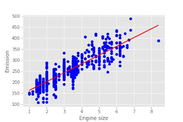
    Coefficient and Intercept in the simple linear regression, are the parameters of the fit line.

print ('Coefficients: ', regr.coef_)
print ('Intercept: ',regr.intercept_)

Out[]:
Coefficients:  [[39.10334822]]
Intercept:  [124.90585427]

    we can plot the fit line over the data,

plt.scatter(train.ENGINESIZE, 
	train.CO2EMISSIONS,
	color='blue')
plt.plot(train_X, 
	reg.coef_[0][0]*train_X + reg.intercept_[0], 
    	'-r')
plt.xlabel("Engine size")
plt.ylabel("Emission")

Model Evaluation

    We compare the actual values and predicted values to calculate the accuracy of a regression model. Evaluation metrics provide a key role in the development of a model, as it provides insight to areas that require improvement.

test_x = np.asanyarray(test[['ENGINESIZE']])
test_y = np.asanyarray(test[['CO2EMISSIONS']])
test_y_hat = regr.predict(test_x)

from sklearn.metrics import r2_score

print("Mean absolute error: %.2f" 
	% np.mean(np.absolute(test_y_hat - test_y)))
print("Residual sum of squares (MSE): %.2f" 
	% np.mean((test_y_hat - test_y) ** 2))
print("R2-score: %.2f" 
	% r2_score(test_y_hat , test_y) )

Out[]:
Mean absolute error: 23.32
Residual sum of squares (MSE): 916.30
R2-score: 0.64

• Mean absolute error: It is the mean of the absolute value of the errors. This is the easiest of the metrics to understand since it’s just average error.
• Root Mean Squared Error (RMSE): This is the square root of the Mean Square Error.
• R-squared is not error, but is a popular metric for accuracy of your model. It represents how close the data are to the fitted regression line. The higher the R-squared, the better the model fits your data. Best possible score is 1.0 and it can be negative (because the model can be arbitrarily worse).

Conclusion:

     In summary, we predicted co2 emission of different cars using simple linear regression on fuel consumption and Carbon dioxide emission of cars data which I have implemented using Scikit learn. If you want to source code, check this GitHub link: Simple linear regression.

Thank you...