Breast Cancer Prediction using CNN

 

Breast Cancer Prediction using Convolutional Neural Network for Beginners

Introduction:

    In this blog, I created Breast Cancer prediction using Convolutional neural network on breast cancer data, which I have implemented using Keras.

    This blog offers you a step-by-step instruction guide with source code, so you can build your model. It is not designed to be a deep dive into model design, statistical analysis, improvement, and validation. If you want to learn more, please check out my blog site: Techy Scientists.

It contains the following parts:

1. Setup your environment
2. Build your Breast Cancer classification model
3. Model Validation
   

Setup your environment

   To run the program on your local computer, install the following required libraries, These libraries are 

1.   python 3.8.0
2.   numpy
3.   pandas
4.   matplotlib
5.   scikit-learn
6.   tensorflow 2.0
7.   keras 2.3.0

Build your Breast Cancer classification model

Step 1: Understand the data

  The first step of model prediction is to understand the data. It is more important to all machine learning and deep learning projects. You can find more information about the data, go to Breast Cancer Data.

Step 2: Import the Packages

  Create a python file (for example model.py). After installed the required packages, import packages  in your python file.

import pandas as pd
import numpy as np
import matplotlib.pyplot as plt
import seaborn as sns

from sklearn import datasets, metrics
from sklearn.model_selection import train_test_split
from sklearn.preprocessing import StandardScaler

from keras import Sequential
from keras.layers import Flatten, Dense, Dropout
from keras.layers import BatchNormalization
from keras.layers import Conv1D, MaxPool1D

Step 3: Import the data

    Next, import the data using pandas

data = datasets.load_breast_cancer()
df = pd.DataFrame(data=data.data, 
	columns=data.feature_names)

Step 4: Split the data

    

    We want to create a model, must have split it into training and testing. the model trained by training dataset and then apply the evaluation of model used by test dataset.

X = df
y = data.target

X_train, X_test, y_train, y_test = 
train_test_split(X, y, test_size=0.2)

print("Train_Data:")
print(X_train.shape)
print(y_train.shape)
print("\nTest_Data:")
print(X_test.shape)
print(y_test.shape)

Out[]:
Train_Data:
(455, 30)
(455,)

Test_Data:
(114, 30)
(114,)

Step 5: Standardization the data

    Standardize the data removes the mean and scales each feature or variable to unit variance.

scaler = StandardScaler()
X_train = scaler.fit_transform(X_train)
X_test = scaler.fit_transform(X_test)

Then, resize the data

X_train = X_train.reshape(455, 30, 1)
X_test = X_test.reshape(114, 30, 1)

Step 6: Create Convolutional Neural Network Model

    We create model for breast cancer prediction model using convolutional neural network. It is type of deep learning networks. It is used for classification, segmentation and image processing problems. In this neural network, extract the features from input layer and perform mathematical convolutional operation. 

epochs = 10
model = Sequential()
model.add(Conv1D(32, 2, 
	activation='relu', 
	input_shape=(30,1)))
model.add(BatchNormalization())
model.add(Dropout(0.2))

model.add(Conv1D(64, 2, activation='relu'))
model.add(BatchNormalization())
model.add(Dropout(0.5))

model.add(Flatten())
model.add(Dense(64, activation='relu'))
model.add(Dropout(0.5))

model.add(Dense(1, activation='sigmoid'))

•     Sequential - appropriate for a plain stack of layers where each layer has    exactly one input tensor and one output tensor.
•     Conv1D - Convolutional one dimensional layer
•     Batch Normalization - allows the network to do learning more independently. It is used to normalize the output of the previous layers.
•     Flatten -  matrix flatten to one dimensional array.
•     Dense - fully connected neural network layer and it implement the operations.
•     Activation - used through an activation  layer, or through the activation argument supported by all forward layers.

Step 7: Train the Model

    Now, we ready to train the model.

model.compile(optimizer='rmsprop', 
	loss='binary_crossentropy', 
    	metrics=['accuracy'])

history=model.fit(X_train,
	y_train,
    	epochs = epochs,
    	validation_data = (X_test, y_test))

Out[]:
Train on 455 samples, validate on 114 samples

Epoch 1/10
455/455 [=========] - 8s 18ms/sample - loss: 0.2800 - 
accuracy: 0.8835- val_loss: 0.4431- val_accuracy: 0.947
Epoch 2/10
455/455 [=========] - 1s 1ms/sample - loss: 0.1105 - 
accuracy: 0.9582- val_loss: 0.3559 - val_accuracy: 0.929
Epoch 3/10
455/455 [=========] - 1s 1ms/sample - loss: 0.1102 - 
accuracy: 0.9648- val_loss: 0.3136 - val_accuracy: 0.886
Epoch 4/10
455/455 [=========] - 1s 1ms/sample - loss: 0.1375 - 
accuracy: 0.9604- val_loss: 0.3360 - val_accuracy: 0.842
Epoch 5/10
455/455 [=========] - 1s 1ms/sample - loss: 0.1137 - 
accuracy: 0.9714- val_loss: 0.3202 - val_accuracy: 0.850
Epoch 6/10
455/455 [=========] - 1s 1ms/sample - loss: 0.0760 - 
accuracy: 0.9802- val_loss: 0.3164 - val_accuracy: 0.842
Epoch 7/10
455/455 [=========] - 1s 1ms/sample - loss: 0.0655 - 
accuracy: 0.9692- val_loss: 0.2960 - val_accuracy: 0.859
Epoch 8/10
455/455 [=========] - 1s 1ms/sample - loss: 0.0661 - 
accuracy: 0.9758- val_loss: 0.3347 - val_accuracy: 0.850
Epoch 9/10
455/455 [=========] - 1s 1ms/sample - loss: 0.1068 - 
accuracy: 0.9758- val_loss: 0.2602 - val_accuracy: 0.877
Epoch 10/10
455/455 [=========] - 1s 1ms/sample - loss: 0.0466 - 
accuracy: 0.9846- val_loss: 0.2348 - val_accuracy: 0.903

Model Validation

    Finally, We created the model and then validate it.

test =  model.evaluate(X_test, y_test, verbose=0)
print("Testing Accuracy: %.2f%%" % (test[1]*100))

Out[]:
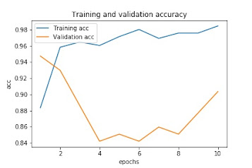
Testing Accuracy: 90.35%

    Visualize the accuracy and loss between training and validation.

def plot_result(history, epoch):
    
    epoch_range = range(1, epoch+1)
    
    plt.plot(epoch_range, 
    	history.history['accuracy'], 
        label='Training acc')
    plt.plot(epoch_range, 
    	history.history['val_accuracy'], 
        label='Validation acc')
    plt.title('Training and validation accuracy')
    plt.xlabel('epochs')
    plt.ylabel('acc')
    plt.legend()

    plt.show()
    
    plt.plot(epoch_range, 
    	history.history['loss'], 
        label='Training loss')
    plt.plot(epoch_range, 
    	history.history['val_loss'], 
        label='Validation loss')
    plt.title('Training and validation loss')
    plt.xlabel('epochs')
    plt.ylabel('loss')
    plt.legend()

    plt.show()

plot_result(history, epochs)

Training and validation accuracy

Training and validation loss

Conclusion:

     In summary, we created the breast cancer prediction model using convolutional neural network on breast cancer data, which I have implemented using Keras. If you want to source code, check this GitHub link: Breast Cancer Prediction using CNN.

Thank you...